Physics Notes - Herong's Tutorial Notes - v3.24, by Herong Yang
Phase Portrait of Pendulum Motion
This section provides phase portrait examples for single object in simple pendulum motion.
Phase portraits of a single object in free fall motion or simple harmonic motion is very simple. Now let's look at phase portraits of a pendulum.
The system of a pendulum can be expressed with a generalized position of one component, q = (θ), where θ is the angular position from the vertical line. So we can express Canonical Coordinates (q,p) of the system as below:
q = (θ)
p = (m*l*l*θ')
  # θ is the angular position from the vertical line
  # m is the mass of the object
  # l is the length of the string
The Hamilton Function can be expressed as:
H = T + V

or:
  H = p*p/(2*m*l*l) + m*g*l(1-cos(q))   (P.9)
If we apply Hamilton Equations, we have:
∂H/∂q = -p'                                (P.2)
∂H/∂p = q'                                 (P.3)

or:
  ∂(p*p/(2m) + k*q*q/2)/∂q = -p'
  ∂(p*p/(2m) + k*q*q/2)/∂p = q'

or:
  m*g*l*sin(q) = -p'                   (P.10)
  p/(m*l*l) = q'                       (P.11)
The Phase Portrait of this system depends on the initial state:
- Ellipse Contour - If you fire the pendulum with a small momentum, it will oscillate around the vertical line.
- Closed Contour - If you fire the pendulum with enough momentum, it will reach the vertical top position with zero momentum, change direction, swing to the vertical top position from the other side, and repeat this pattern.
- Open Contour - If you fire the pendulum with too much momentum, it will reach the vertical top position with some momentum, pass the position, come down on the other side, and continue the circular motion is the same direction without oscillation.
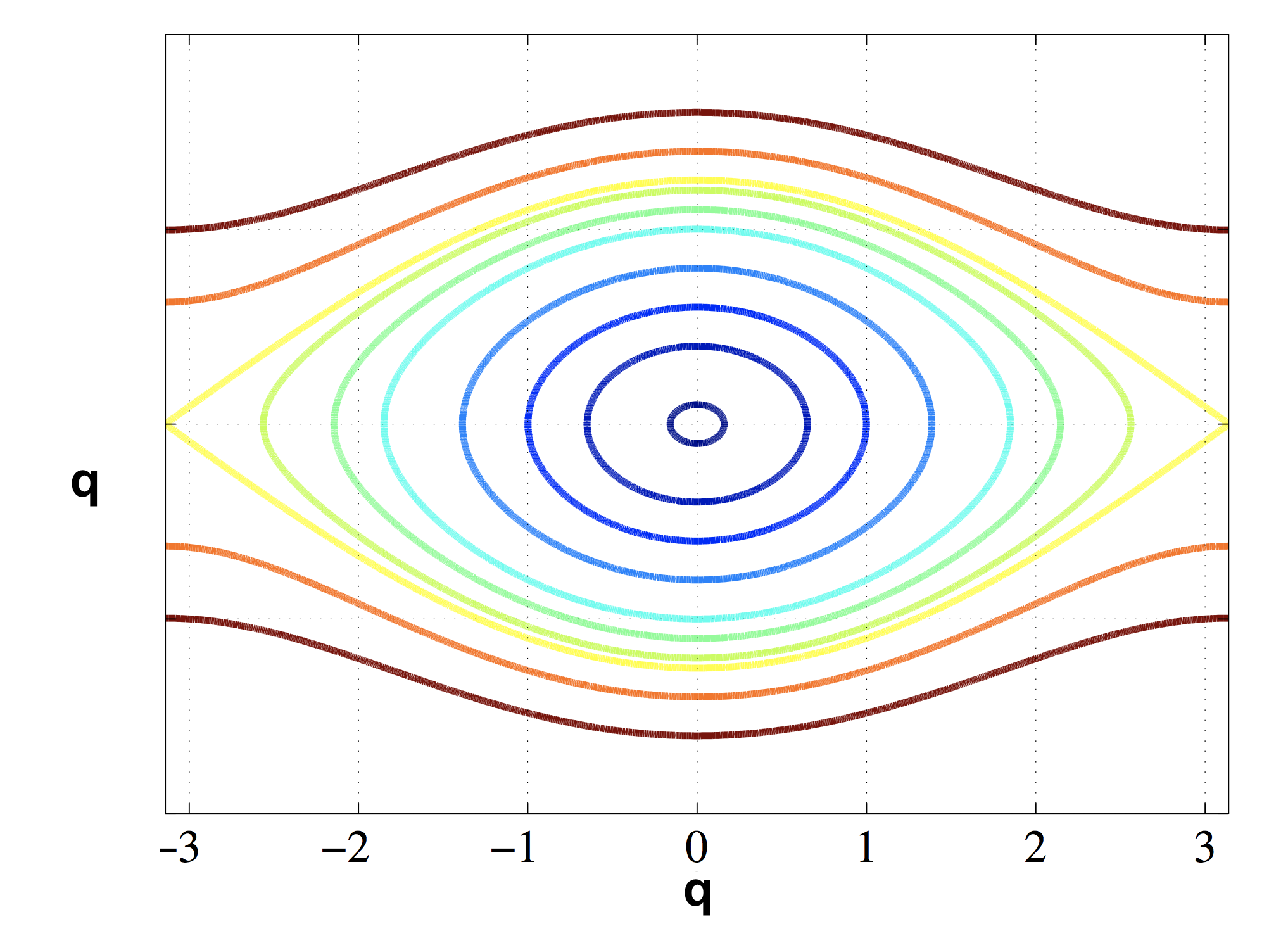
Table of Contents
Introduction of Frame of Reference
Introduction of Special Relativity
Time Dilation in Special Relativity
Length Contraction in Special Relativity
The Relativity of Simultaneity
Minkowski Spacetime and Diagrams
Introduction of Generalized Coordinates
►Phase Space and Phase Portrait
Phase Portrait of Simple Harmonic Motion
►Phase Portrait of Pendulum Motion
Motion Equations of Linear Systems