Phase Portraits of 2-D Homogeneous Linear Systems

∟Phase Portraits of 2-D Homogeneous Linear Systems

This section provides a quick introduction on classifications of phase portraits of 2-D homogeneous linear systems based on characteristic polynomials of their linear coefficient matrixes.

What Is 2-D Linear System? A 2-D Linear System is a single-object system with 1 degree of freedom and it's motion equations are first order linear differential equations of the canonical coordinates.

As we see in the last tutorial, the motion equations can be expressed in vector form as:

x' = Ax + b                            (P.12)

where: 
  x = |q|
      |p|
  x' = |q'|
       |p'|
  A = |a₁₁, a₁₂|
      |a₂₁, a₂₂|
  b = |b₁|  
      |b₂|

What Is Homogeneous Linear System? A Homogeneous Linear System is a special linear system where all constant terms are zero in the motion equations:

x' = Ax                                (P.13)

since: 
  x' = Ax + b                          (P.12)
  b is a zero vector

The above motion equations can be viewed as that the time derivatives of the canonical coordinates is a linear transformation of the canonical coordinates, where A is called the transformation matrix.

What Is 2-D Homogeneous Linear System? A 2-D Homogeneous Linear System is the simplest motion system, where the motion equations can be expressed in vector form as:

x' = Ax                                (P.13)

where: 
  A = |a₁₁, a₁₂|
      |a₂₁, a₂₂|

Classification of 2-D Homogeneous Linear Systems

Since 2-D homogeneous linear systems are governed by 2-D matrixes, they can be classified based on characteristic polynomials of their 2-D matrixes.

x' = Ax                                (P.13)
p(r) = r² - c*r + d                    (P.14)

where:
  p(r) is the characteristic polynomial
  r is an eigenvalue of A
  c = a₁₁ + a₂₂
  d = a₁₁*a₂₂ - a₁₂*a₂₁ 
  A = |a₁₁, a₁₂|
      |a₂₁, a₂₂|

The roots of the characteristic polynomial are called eigenvalues of matrix A. And the types of roots are determined by the discriminant of the characteristic polynomial:

discriminant = c² - 4*d
eigenvalues = (c +|- sqrt(discriminant))/2
  r₁ = (c + sqrt(discriminant))/2
  r₂ = (c - sqrt(discriminant))/2

cases:
  1: Discriminant > 0 with 2 real eigenvalues
  2: Discriminant < 0 with 2 complex eigenvalues
  3: Discriminant = 0 with 1 real eigenvalue (double eigenvalues)

Case 1: Discriminant > 0 with 2 Real Eigenvalues - There are 3 subcases when the discriminant is positive:

Subcases: 
  1.1: Nodal source with 2 positive eigenvalues
  1.2: Saddle with 1 positive eigenvalue and 1 negative eigenvalue
  1.3: Nodal sink (attractor) with 2 negative eigenvalues

In Case 1, there are 4 half straight-line trajectories corresponding to the eigenvectors of matrix A. See next chapter for more details on eigenvectors.

Each half straight-line trajectory is either moving toward or away from the origin of the phase plane.

Other trajectories are curves located in 4 regions separated by the 4 half straight-line trajectories.

Subcase 1.1: Nodal Source with 2 Positive Eigenvalues - In this case, all trajectories are moving away from the origin of the phase plane. See the illustration below (source: math.colostate.edu):

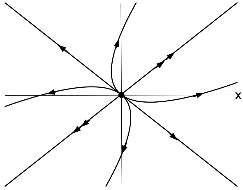
2-D Phase Portrait Pattern - Nodal Source

Subcase 1.2: Saddle with 1 Positive Eigenvalue and 1 Negative Eigenvalue - In this case, 2 half straight-line trajectories are moving away from the origin, and 2 other half straight-line trajectories are moving toward the origin. All other trajectories are not passing the origin. See the illustration below (source: math.colostate.edu):

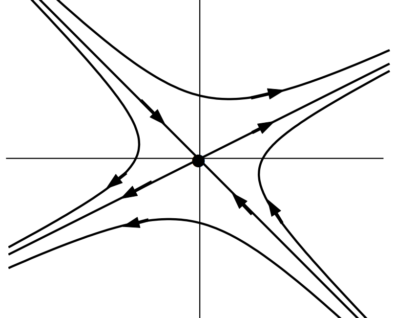
Subcase 1.3: nodal Sink (Attractor) with 2 Negative Eigenvalues - In this case, all trajectories are moving toward the origin. See the illustration below (source: math.colostate.edu):

Case 2: discriminant < 0 with 2 complex eigenvalues - In this case, eigenvalues can be expressed as:

  r₁ = 0.5*c + 0.5*sqrt(-discriminant)*i  
  r₂ = 0.5*c - 0.5*sqrt(-discriminant)*i

There are 3 subcases based on the sign of the real component, c, of the eigenvalues:

Subcases: 
  2.1: Spiral source (growing oscillations) with c > 0 
  2.2: Center (closed curves) with c = 0
  2.3: Spiral sink (decaying oscillations) with c < 0

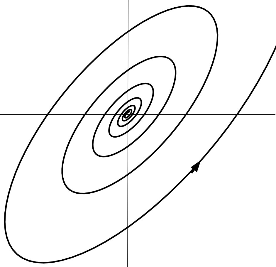
Subcase 2.1: Spiral Source with c > 0 - In this case, all trajectories are moving away from the origin of the phase plane as spiral curves. See the illustration below (source: math.colostate.edu):

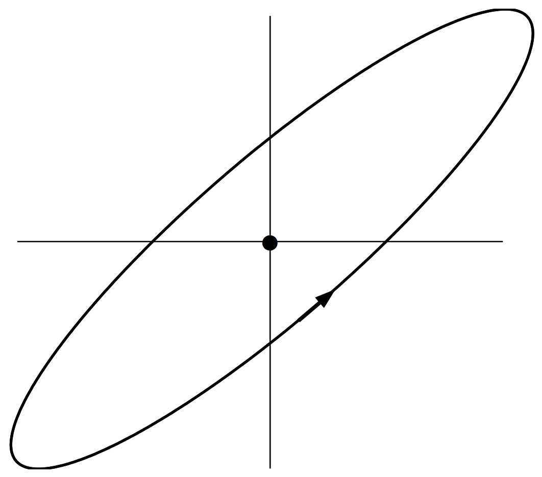
2-D Phase Portrait Pattern - Spiral Source

Subcase 2.2: Center with c = 0 - In this case, all trajectories are closed eclipses centering at the origin. See the illustration below (source: math.colostate.edu):

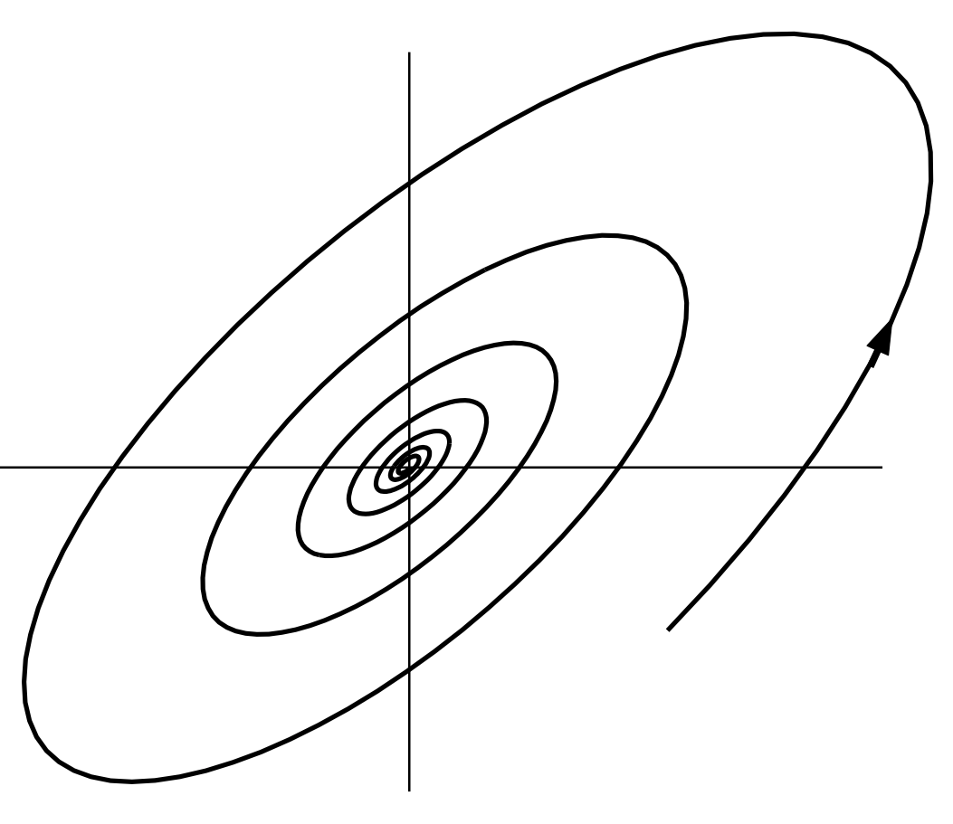
Subcase 2.3: Spiral Sink with c < 0 - In this case, all trajectories are toward the origin as spiral curves. See the illustration below (source: math.colostate.edu):

2-D Phase Portrait Pattern - Spiral Sink

Case 3: discriminant = 0 with 1 Real Eigenvalue - In this case, the eigenvalue can be expressed as:

  r₁ = r₂ = 0.5*c

And there can be 1 or 2 linearly independent eigenvectors.

There are 4 subcases based on the sign of the real component, c, of the eigenvalue and the number of linearly independent eigenvectors:

Subcases: 
  3.1: Proper nodal source with c < 0 and 2 eigenvectors
  3.2: Proper nodal sink with c > 0 and 2 eigenvectors
  3.3: Improper nodal source with c < 0 and 1 eigenvector
  3.4: Improper nodal sink with c > 0 and 1 eigenvector

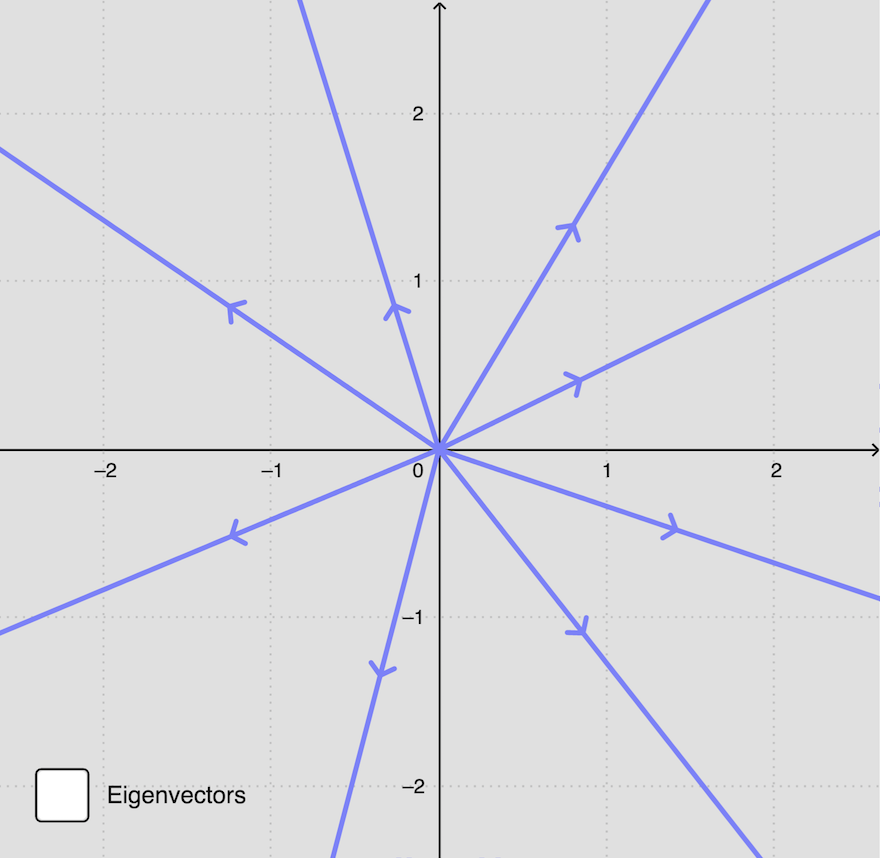
Subcase 3.1: Proper nodal source with c < 0 and 2 eigenvectors - This case is also called singular nodal source, where all trajectories are moving away from the origin of the phase plane as half straight-lines. See the illustration below (source: geogebra.org):

2-D Phase Portrait Pattern - Proper Nodal Source

Subcase 3.2: Proper nodal sink with c > 0 and 2 eigenvectors - This case is also called singular nodal sink, where all trajectories are moving toward the origin as half straight-lines. See the illustration below (source: geogebra.org):

2-D Phase Portrait Pattern - Proper Nodal Sink

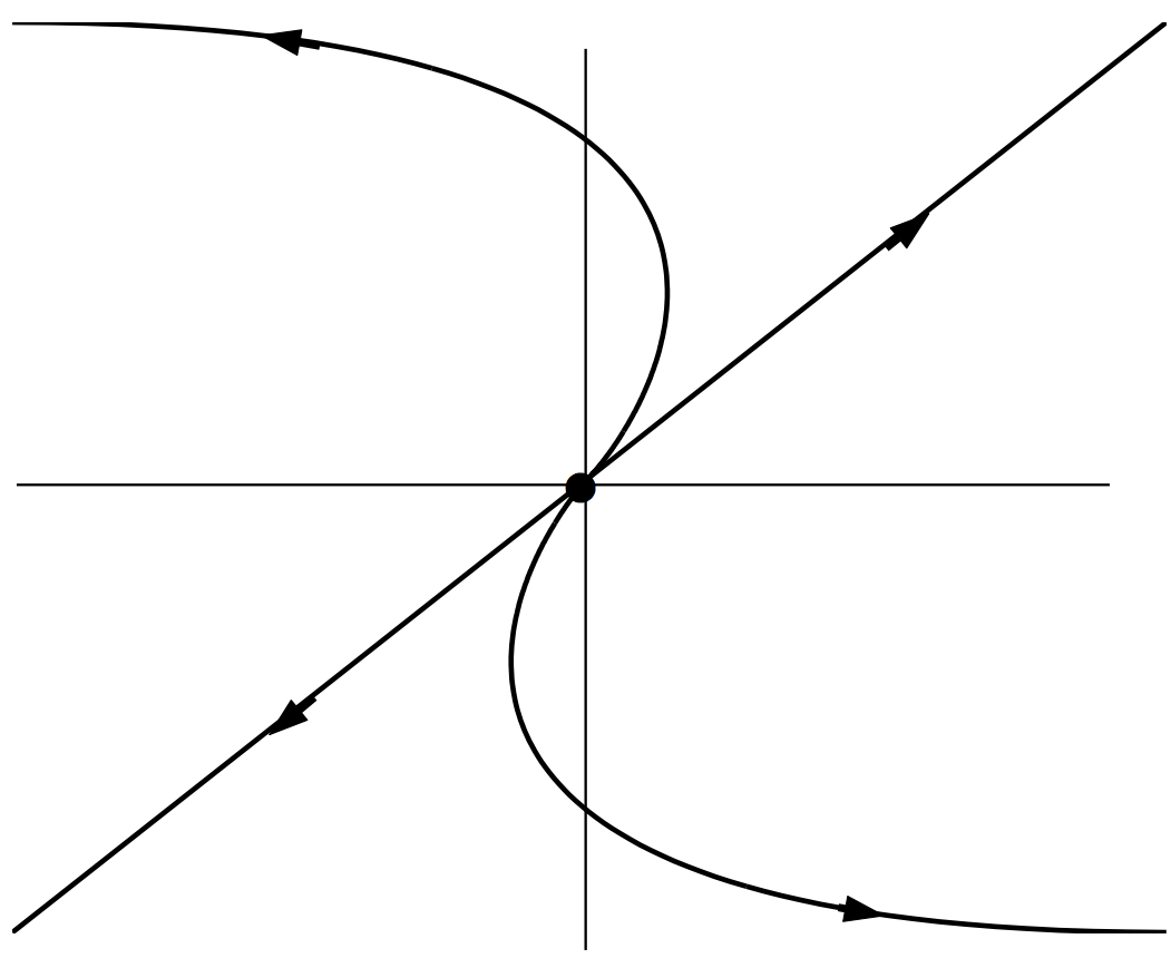
Subcase 3.3: Improper nodal source with c < 0 and 1 eigenvector - This case is also called degenerate nodal source, where all trajectories are moving away from the origin. 2 of them are half straight-line trajectories. See the illustration below (source: math.colostate.edu):

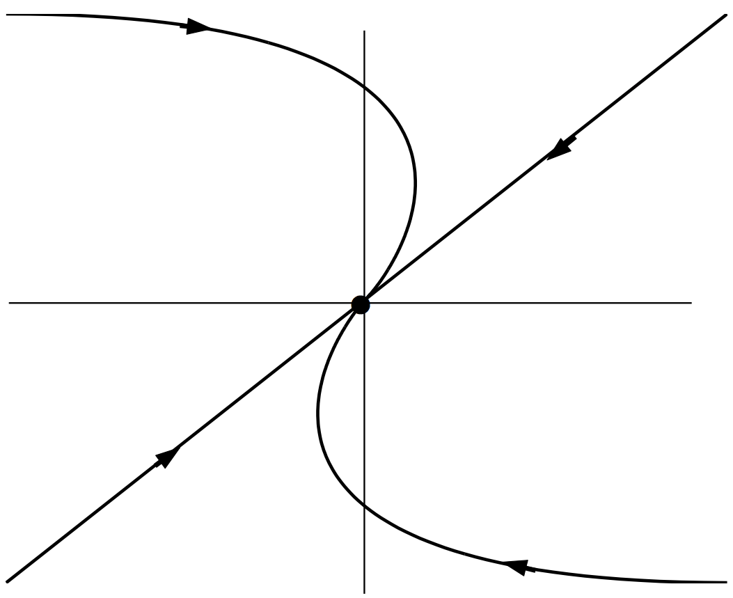
2-D Phase Portrait Pattern - Improper Nodal Source

Subcase 3.4: Improper nodal sink with c > 0 and 1 eigenvector - This case is also called degenerate nodal sink, where all trajectories are moving toward the origin. 2 of them are half straight-line trajectories. See the illustration below (source: math.colostate.edu):