Physics Notes - Herong's Tutorial Notes

∟Introduction of Lagrangian

∟Action - Functional of Position Function x(t)

This section describes the Action S as a functional of position function x(t).

In the last section, we defined a very important concept of a mechanical system, Action S, as the integral of Lagrangian L(t) between two time instances.

S = ∫ L(t)dt between t1 and t2      (G.2)
  # L(t) is Lagrangian of the system.

If we consider a system with a single moving object, the position of the object is a function of time, x(t). And its velocity is also a function of time, x'(t). In this case, Lagrangian can also be expressed as a function of t, x(t) and x'(t):

L = L(x,x',t)                      (G.1)
  # x, shorthand of x(t), is the position of the object
  # x', shorthand of x'(t), is the velocity of the object

Of course, in the real physical world, the object will move according to a fixed function x(t) from the starting point x(t₁) to the ending point x(t₂).

If the position function x(t) is fixed, the velocity function x'(t) is also fixed. So the Lagrangian function depends on a single variable, time t. And the Action S becomes a fixed value.

S = ∫ L(t)dt between t1 and t2      (G.2)
  # S is fixed, if x(t) is fixed based on physical laws

However, if the object does not follow any physical law, it can, mathematically, move according to any function x(t) that connects x(t₁) and x(t₂).

In other words, the object can take any path in spacetime, moving from the starting point x(t₁) to the ending point x(t₂). For each different path x(t), we will have a different Lagrangian function L(x,x',t).

So mathematically, Action S is not a constant any more. It is a functional of x(t), expressed as:

S = S[x(t)]

or:
  S[x(t)] = ∫ L(x,x',t)dt           (G.2)
    # x(t) is any mathematical function

If the object moves in a straight line, the position function x(t) has only 1 component, represented by x. In this can, we can plot any position function x(t) in 2-dimensional plane of (t,x).

The following diagram shows 3 examples of position functions on the (t,x) plane between two time instances, t₁ and t₂, they may look: (source: slideplayer.com)

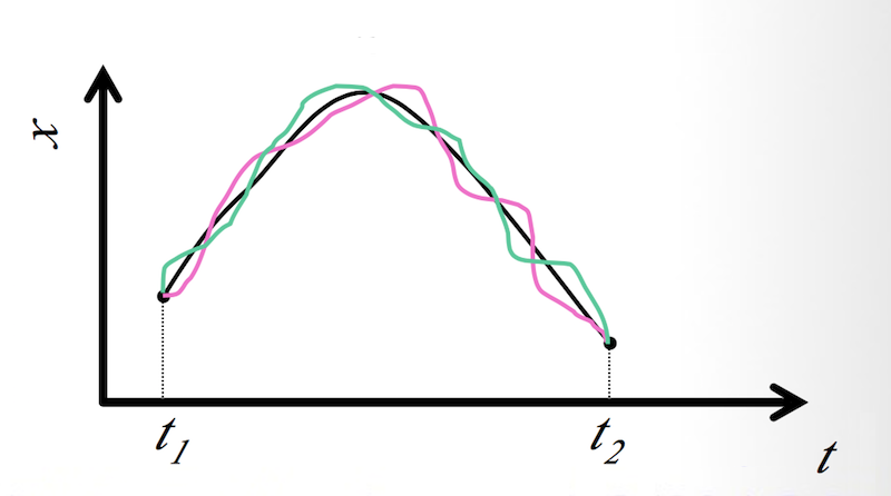
Those 3 position functions are plotted in 3 colors: black, pink and green: x_black, x_pink and x_green, will result 3 Lagrangian functions: L_black, L_pink and L_green.

Lblack(t) = L(xblack,x'black,t)
Lpink(t)  = L(xpink, x'pink ,t)
Lgreen(t) = L(xgreen,x'green,t)

Those 3 Lagrangian functions will then result 3 Action values: S_black, S_pink and S_green.

Sblack = ∫ Lblack(t)dt
Spink  = ∫ Lpink(t)dt
Sgreen = ∫ Lgreen(t)dt

or:
Sblack = S[xblack(t)]
Spink  = S[xpink(t)]
Sgreen = S[xgreen(t)]

Mathematically, there are infinite number of functions x(t) that meet the boundary conditions of the two ending points (t₁, x₁) and (t₂, x₂). So S[x(t)] is a functional, a function of functions x(t).

Now we should have a good understanding of what is Action S, and why it is called a functional of x(t).

Table of Contents

 About This Book

 Introduction of Space

 Introduction of Frame of Reference

 Introduction of Time

 Introduction of Speed

 Newton's Laws of Motion

 Introduction of Special Relativity

 Time Dilation in Special Relativity

 Length Contraction in Special Relativity

 The Relativity of Simultaneity

 Introduction of Spacetime

 Minkowski Spacetime and Diagrams

 Introduction of Hamiltonian

►Introduction of Lagrangian

 What Is Lagrangian

 Action - Integral of Lagrangian

►Action - Functional of Position Function x(t)

 Hamilton's Principle - Stationary Action

 What Is Lagrange Equation

 Other Proofs of the Lagrange Equation

 Lagrange Equation on Free Fall Motion

 Lagrange Equation on Simple Harmonic Motion

 Lagrangian in Cartesian Coordinates

 Lagrange Equations in Cartesian Coordinates

 Introduction of Generalized Coordinates

 Phase Space and Phase Portrait

 References

 Full Version in PDF/ePUB

Action - Functional of Position Function x(t) - Updated in 2022, by Herong Yang